Zhang K., Li D. Electromagnetic Theory for Microwaves and Optoelectronics

Подождите немного. Документ загружается.

6.8 Dielectric Resonators 391

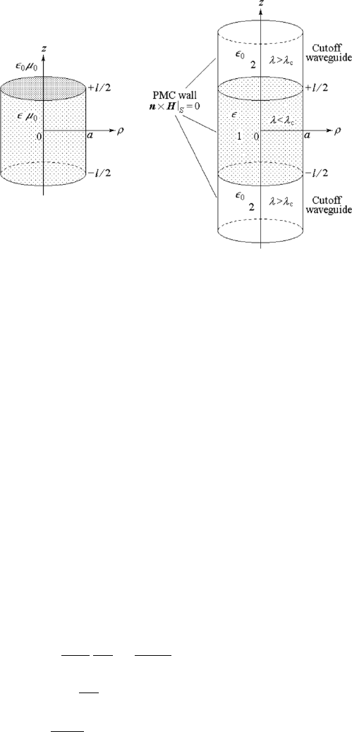
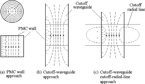
Figure 6.28: Cutoﬀ-waveguide approach for a dielectric resonator.

6.8.2 Cutoﬀ-Waveguide Approach

In the PMC wall model, all the ﬁelds outside the dielectric object are ne-

glected. In the improved model, the dielectric resonator is seen as a circular

waveguide with an open-circuit wall at ρ = a. In the waveguide, a segment of

length l is ﬁlled with a dielectric, with ², which is the resonator, and beyond

the ends of the resonator, the waveguide either has vacuum inside or is ﬁlled

with air. See Fig. 6.28. The ﬁelds outside the cylinder of radius a are again

neglected, and the ﬁelds inside the cylinder of radius a are taken into account.

In region 1, |z| ≤ l/2, i.e., inside the resonator, the waveguide is in a guiding

state and the ﬁelds are standing waves along z. In region 2, |z| ≥ l/2, and

ρ ≤ a, i.e., outside the resonator but inside the waveguide, the waveguide is

in a cutoﬀ state and the ﬁelds are decaying ﬁelds along +z and −z.

For TE modes, the V function and the ﬁeld expressions in region 1 are

the same as those in the PMC wall model,

= AJ

(T ρ) cos nφ cos(βz + θ), (6.347)

ρ1

= −

jωµ

∂V

∂φ

jωµ

(T ρ) sin nφ cos(βz + θ), (6.348)

φ1

= jωµ

∂V

∂ρ

= jωµ

T AJ

(T ρ) cos nφ cos(βz + θ), (6.349)

ρ1

∂

∂ρ ∂z

= −βT AJ

(T ρ) cos nφ sin(βz + θ), (6.350)

392 6. Dielectric Waveguides and Resonators

φ1

∂

∂φ ∂z

βn

(T ρ) sin nφ sin(βz + θ), (6.351)

= T

V = T

(T ρ) cos nφ cos(βz + θ)., (6.352)

In region 2, the V function and the ﬁelds of cutoﬀ modes are given by

= BJ

(T ρ) cos nφ e

−α(|z|−l/2)

, (6.353)

ρ2

jωµ

(T ρ) sin nφ e

−α(|z|−l/2)

, (6.354)

φ2

= jωµ

T BJ

(T ρ) e

−α(|z|−l/2)

, (6.355)

ρ2

= −αT BJ

(T ρ) cos nφ e

−α(|z|−l/2)

, (6.356)

φ2

αn

(T ρ) sin nφ e

−α(|z|−l/2)

, (6.357)

= T

(T ρ) cos nφ e

−α(|z|−l/2)

. (6.358)

The relations between β, α, and T are given by

+ T

= k

= ω

², −α

+ T

= k

= ω

. (6.359)

The boundary conditions on the side of the waveguide, ρ = a, are again

(a) = 0 and H

(a) = 0, which give

(T a) = 0, T

. (6.360)

At the end surfaces, |z| = ±l/2, the tangential component of the ﬁelds must

be continuous, which gives

φ1

(±l/2) = E

φ2

(±l/2)

ρ1

(±l/2) = E

ρ2

(±l/2)

→ A cos(βl/2 + θ) = B,

φ1

(±l/2) = H

φ2

(±l/2)

ρ1

(±l/2) = H

ρ2

(±l/2)

→ βA sin(βl/2 + θ) = αB.

Subtracting the above two equations and canceling A and B, we have

β tan(βl/2 + θ) = α. (6.361)

Considering the symmetry property of the resonator, we know that the ﬁelds

must be either even symmetrical or odd symmetrical, i.e.,

θ = 0, for even modes, or θ = π/2, for odd modes,

and (6.361) becomes

β tan(βl/2) = α, β tan(βl/2 + π/2) = α.

6.8 Dielectric Resonators 393

Then we have

βl = 2 arctan(α/β)+pπ =(p+δ)π,

p=0, 2, 4, ···, for even modes,

p=1, 3, 5, ···, for odd modes,

(6.362)

where

δ =

2 arctan(α/β)

. (6.363)

The modes of the resonator is denoted by TE

n,m,p+δ

and the natural

angular frequency is given by

n,m,p+δ

+ T

[(p + δ)π/l]

+ (x

/a)

. (6.364)

For the dominant TE mode, the TE

01δ

mode, with n = 0, m = 1, p =

0, β = δπ/l, we have

T =

2.405

, βl =2 arctan

, β =

²−T

, α =

−ω

(6.365)

The solution of TM modes can also be obtained by means of the cutoﬀ-

waveguide terminal approach, which we leave as a problem for the reader.

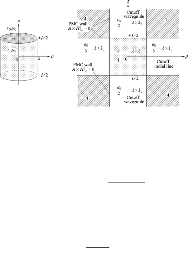
6.8.3 Cutoﬀ-Waveguide, Cutoﬀ-Radial-Line Approach

To obtain the exact solution, the whole space needs to be separated into four

regions, shown in Fig. 6.29. In region 1, ρ ≤ a, |z| ≤ ±l/2, i.e., inside the

resonator, the ﬁelds are standing waves in both the ρ and the z direction. In

regions 2, ρ ≤ a, |z| ≥ ±l/2, i.e., beyond the end surfaces of the resonator, the

ﬁelds are standing waves in the ρ direction and are decaying ﬁelds in the ±z

direction. In region 3, ρ ≥ a, |z| ≤ ±l/2, i.e., outside the side surfaces of the

resonator, the ﬁelds are standing waves in the z direction and are decaying

ﬁelds in the ρ direction. Finally, in regions 4, ρ ≥ a, |z| ≥ ±l/2, the ﬁelds

that are decaying in both the ρ and the z direction can be neglected. The

physical model used by the approach is such that beyond the end surfaces

of the resonator lay the cutoﬀ waveguides with perfect magnetic walls and

outside the side surface there should be a cutoﬀ radial line. Therefore, this

approach is known as the cutoﬀ-waveguide, cutoﬀ-radial-line approach. We

are devoted to the circumferential uniform modes for which n = 0.

For TE modes, the V functions in the three regions are given by

= AJ

(T ρ) cos βz, (6.366)

= BJ

(T ρ)e

−α(|z|−l/2)

, (6.367)

= CK

(τρ) cos βz, (6.368)

where

+ T

= k

= ω

², −α

+ T

= k

= ω

, β

−τ

= k

= ω

394 6. Dielectric Waveguides and Resonators

Figure 6.29: Cutoﬀ-waveguide, cutoﬀ-radial-line approach for a dielectric

resonator.

The boundary conditions on the end surfaces are the same as those for

the cutoﬀ-waveguide approach in the last subsection, and we have

βl = (p + δ)π, δ =

2 arctan(α/β)

From the boundary conditions on the side surface of the cylinder, ρ = a,

φ1

(a) = E

φ3

(a) → T AJ

(T a) = τ CK

(τa),

(a) = H

(a) → T

(T a) = −τ

(τa),

we get

C =

T J

(T a)

τK

(τa)

A, (6.369)

and

T aJ

(T a)

= −

τaK

(τa)

. (6.370)

This is the eigenvalue equation for the TE

0,m,p+δ

modes for circular cylindri-

cal dielectric resonator. It is similar to that of the circular dielectric waveg-

uide.

The sketch drawings of the electric and magnetic ﬁelds obtained from

the above three approaches on a circular cylindrical dielectric resonator are

shown in Fig. 6.30.

6.8 Dielectric Resonators 395

Figure 6.30: Sketch maps of the electric and magnetic ﬁelds for the TE

0,1,δ

mode in a circular cylindrical dielectric resonator.

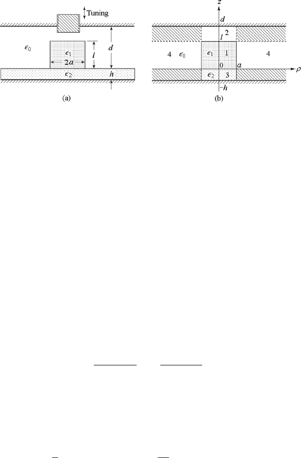
6.8.4 Dielectric Resonators in Microwave Circuits

In microwave integrated circuits or strip-line circuits, the dielectric resonator

is practically mounted on a dielectric substrate with much lower permittivity

than that of the resonator. Below the substrate and on top of the resonator,

metallic plates are placed for use as the casing. See Fig. 6.31a. The p ermit-

tivity of the resonator, region 1, is ²

, the permittivities of regions 2 and 4

are ²

, and the permittivity of region 3 is ²

, ²

< ²

¿ ²

. See Figure 6.31b.

For TE modes, the V functions and the ﬁeld components in the four

regions are given by

= AJ

(T ρ) sin(βz + θ), (6.371)

φ1

= −jωµ

T AJ

(T ρ) sin(βz + θ), (6.372)

ρ1

= −βT AJ

(T ρ) cos(βz + θ), (6.373)

= T

(T ρ) sin(βz + θ), (6.374)

= BJ

(T ρ) sinh[α

(d − z)], (6.375)

φ2

= −jωµ

T BJ

(T ρ) sinh[α

(d − z)], (6.376)

ρ2

= α

T BJ

(T ρ) cosh[α

(d − z)], (6.377)

= T

(T ρ) sinh[α

(d − z)], (6.378)

= CJ

(T ρ) sinh[α

(z + h)], (6.379)

φ3

= −jωµ

T CJ

(T ρ) sinh[α

(z + h)], (6.380)

ρ3

= −α

T CJ

(T ρ) cosh[α

(z + h)], (6.381)

= T

(T ρ) sinh[α

(z + h)], (6.382)

396 6. Dielectric Waveguides and Resonators

Figure 6.31: Practical dielectric resonator in microwave integrated circuits.

= DK

(τρ) sin(βz + θ), (6.383)

φ4

= −jωµ

τDK

(τρ) sin(βz + θ), (6.384)

ρ4

= −βτ DK

(τρ) cos(βz + θ), (6.385)

= τ

(τρ) sin(βz + θ), (6.386)

where

+ T

= k

= ω

², (6.387)

− τ

= k

= ω

, (6.388)

−α

+ T

= k

= ω

, (6.389)

−α

+ T

= k

= ω

. (6.390)

Applying the argument that the boundary condition on the side surface,

ρ = a is such that tangential components of both electric and magnetic ﬁelds

are continuous, we have the same eigenvalue equation as that in the last

subsection:

T aJ

(T a)

= −

τaK

(τa)

. (6.391)

Applying the argument that the boundary condition on the top-end surface,

z = l, we write E

φ1

(l) = E

φ2

(l) and H

ρ1

(l) = H

ρ2

(l), which immediately

gives

β cot(βl + θ) = α

coth[α

(d − l)],

and then

− (βl + θ) = arctan

coth[α

(d − l)]

. (6.392)

Applying the same argument about the boundary condition on the bottom-

end surface, z = 0 as on the top-end surface, we write E

φ1

(0) = E

φ2

(0) and

ρ1

(0) = H

ρ2

(0), which gives

β cot θ = −α

coth(α

h), (6.393)

Problems 397

− θ = −arctan

coth(α

. (6.394)

From (6.392), (6.393) and (6.394), it follows that

βl = arctan

coth[α

(d − l)]

+ arctan

coth(α

+ pπ. (6.395)

The natural angular frequency of the resonator is then found from equa-

tions (6.387), (6.389), (6.391), and (6.395). It can be seen that the natural

frequency of the resonator is determined not only by the size of the resonator

but also by the spacing d −l. Hence the resonator can be tuned by adjusting

a bolt on the top cover of the casing.

Problems

6.1 Show that the boundary conditions of the waveguide shown in Fig. 6.1b

can be satisﬁed by the ﬁelds of LSE

(y )

or LSM

(y )

modes.

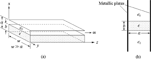
6.2 Find the ﬁelds and the propagation characteristics of the parallel-plate

transmission line, partially ﬁlled with dielectric material, shown in

Fig. 6.32(a). Suppose that the widths of the plates are much larger

than the spacing between the plates.

6.3 Find the change in the cutoﬀ frequency due to ﬁlling of dielectric in the

metallic waveguide shown in Fig. 6.1a by using the method of perturba-

tion. Compare the result with that of the ﬁeld analysis in Section 6.1.

6.4 A dielectric waveguide made of high permittivity material (for example

> 30) can be analyzed approximately by means of the open-circuit

boundary model. Find the ﬁeld components, eigenvalue equation, and

the propagation characteristics of a rectangular waveguide enclosed by

open-circuit boundaries. Show that this is the dual problem of the

metallic waveguide.

6.5 Find the ﬁeld components, eigenvalue equation, and the propagation

characteristics of a circular waveguide enclosed by open-circuit bound-

aries. Show that it is the dual problem of the metallic waveguide.

6.6 Find the ﬁeld components, eigenvalue equation, and the propagation

characteristics of the rectangular waveguide, in which the wide walls

are approximately open-circuit planes and the narrow walls are approx-

imately short-circuit planes. It is the large permittivity approximation

of the dielectric H-type waveguide given in the next problem.

398 6. Dielectric Waveguides and Resonators

Figure 6.32: (a) Problem 6.2. Parallel-plate line, partially ﬁlled with dielec-

tric material, (b) Problem 6.7. H-type waveguide.

6.7 Find the ﬁeld components, eigenvalue equation, and the propagation

characteristics of the H-type waveguide shown in Fig. 6.32(b). Suppose

the permittivity of the dielectric is not very large.

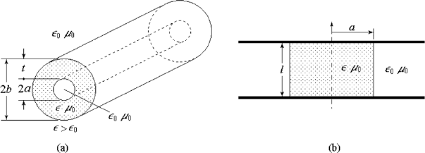
6.8 Find the ﬁeld components, eigenvalue equation, and the propagation

characteristics of the circularly symmetric TE and TM modes in the

circular dielectric tube shown in Figure 6.33(a).

6.9 Find the ﬁeld components, eigenvalue equation, and the propagation

characteristics of the circularly symmetric TM modes in the circular

metallic waveguide coated with a dielectric layer on the inner wall. The

inner radius of the waveguide is a, the inner radius of the dielectric layer

is b and the permittivity of the dielectric material is ².

6.10 Show that for axial asymmetrical, i.e., angular nonuniform ﬁelds, the

TE or TM modes alone cannot satisfy the dielectric boundary condi-

tions of waveguides given in Problems 6.8, 6.9 and Section 6.7.

6.11 For the case when the permittivity of the dielectric is very large

(²

> 30), repeat problem 6.8 by using the model of a perfect mag-

netic conducting wall and compare the results with those found for the

coaxial line.

6.12 Find the ﬁelds and the natural frequencies of the TM modes of a circular

cylindrical dielectric resonator by using the cutoﬀ-waveguide approach.

6.13 Find the ﬁelds and the natural frequencies of a circular cylindrical di-

electric resonator between two metallic plate at the two ends. Suppose

the permittivity of the dielectric is very large. Refer to Fig. 6.33(b).

6.14 Repeat the last problem for the case when the permittivity of the di-

electric is not very large.

Problems 399

Figure 6.33: (a) Problem 6.8. Circular dielectric tube, (b) Problem 6.13.

Cylindrical dielectric resonator between two metallic plate.

6.15 A dielectric cylinder of radius b and permittivity ² is inserted in a

cylindrical cavity with radius a and length l along the axis. Find the

natural frequency of the TM

010

mode and compare the result to that

of problem 5.17.

6.16 (1) Derive the eigenvalue equation and the ﬁeld components of the TE

modes for an asymmetrical planar dielectric waveguide by using the

ﬁeld-matching method.

(2) Derive the eigenvalue equation and the ﬁeld components of the TM

modes for an asymmetrical planar dielectric waveguide by using the

impedance-matching method.

6.17 An asymmetrical dielectric slab waveguide is constructed by growing

a GaAs layer on the AlGaAs substrate. The index of the AlGaAs

substrate is n

= 3.5, that of the GaAs guiding layer is n

= 1.03n

and the cladding is air, n

= 1. Find the maximum thickness of the

guiding layer so that the waveguide operating in single-mode state for

the wavelength larger than λ = 1 µm.

6.18 A single-mode optical ﬁber is made of fused silica, the refraction indices

of the cladding and the core are n

= 1.518 and n

= 1.015n

= 1.541,

respectively, and the diameter of the core is 2a = 4 µm. Find the cutoﬀ

wavelength of the mo de next to the dominant mode.

6.19 (1) Find the maximum radius of a single-mode optical ﬁber operating

at wavelength 1.3µm. The ﬁber is made of the same material as that

of the last problem.

(2) Repeat the last question for a multi-mode optical ﬁber with 50

modes propagating in the ﬁber.

400 6. Dielectric Waveguides and Resonators

6.20 Find the ﬁeld components and eigenvalue equations for the x linear

polarized modes in a weekly guiding optical ﬁber.

6.21 Prove that the ﬁelds with single space harmonic cannot satisfy the exact

boundary conditions for a circular cylindrical dielectric resonator, as it

doesn’t for rectangular dielectric waveguide.

6.22 Show that, if the operating frequency is much higher than the cutoﬀ

frequency, ω À ω

, τa → ∞, then the parameter χ of circular dielectric

waveguide is equal to +1 for EH modes and −1 for HE modes, and

the transverse ﬁelds in weakly guiding circular dielectric waveguide are

circularly polarized.

EH (χ = +1) HE (χ = −1)

ρ1

= jk

T AJ

n+1

(T ρ)e

jnφ

−jβz

−jk

T AJ

n−1

(T ρ)e

jnφ

−jβz

φ1

= k

T AJ

n+1

(T ρ)e

jnφ

−jβz

T AJ

n−1

(T ρ)e

jnφ

−jβz

= T

(T ρ)e

jnφ

−jβz

(T ρ)e

jnφ

−jβz

ρ1

= −(k

/η

)T AJ

n+1

(T ρ)e

jnφ

−jβz

−(k

/η

)T AJ

n−1

(T ρ)e

jnφ

−jβz

φ1

= j(k

/η

)T AJ

n+1

(T ρ)e

jnφ

−jβz

−j(k

/η

)T AJ

n−1

(T ρ)e

jnφ

−jβz

= j(1/η

(T ρ)e

jnφ

−jβz

−j(1/η

(T ρ)e

jnφ

−jβz