Klipp E., Herwig R., Kowald A., Wierling C., Lehrach H. Systems Biology in Practice: Concepts, Implementation and Application

Подождите немного. Документ загружается.

bridization experiment (Poustka et al. 1986), using this, among other applications, to

determine transcript levels for many genes in parallel. Since then, several array plat-

forms have been developed and a vast number of studies have been conducted. The

principle of these techniques is the same (cf. Chapter 4): large numbers of probes

(typically on the order of 10,000) are immobilized on a solid surface and hybridiza-

tion experiments with a complex pool of labeled RNAs are performed. After attach-

ing to the reverse complementary sequence, the amount of bound labeled material

is quantified by a scanning device and is transformed into a numerical value that re-

flects the abundance of the specific probe in the RNA pool. The different technolo-

gies differ in the material of the solid support, the labeling procedure, and the nature

of the probes.

Historically, macroarrays were the first DNA array platform. This technique, devel-

oped in the late 1980s (Poustka et al. 1986; Lehrach et al. 1990; Lennon and Lehrach

1991), employs PCR products of cDNA clones that are immobilized on nylon filter

membranes. The mRNA target material is labeled radioactively (

P) by reverse tran-

scription. cDNA macroarrays typically have a size of 8612 cm

to 22622 cm

and

cover up to 80,000 different cDNAs. The bound radioactivity is detected using a

phosphor imager. Multiple studies using this technique have been published (Gress

et al. 1992, 1996; Granjeaud et al. 1996; Nguyen et al. 1996; Dickmeis et al. 2001;

Kahlem et al. 2004).

Another platform is microarrays. Here, cDNA sequences are immobilized on glass

surfaces and hybridizations are carried out with fluorescently labeled target material.

Chips are small (1.861.8 cm

) and allow the spotting of tens of thousands of differ-

ent cDNA clones. cDNA microarrays are widely used in genome research (Schena

et al. 1995, 1996; DeRisi et al. 1996, 1997; Spellman et al. 1998; Iyer et al. 1999; Bitt-

ner et al. 2000; Whitfield et al. 2002). A specific advantage of this technology is the

fact that two RNA samples labeled with different dyes can be mixed within the same

hybridization experiment (cf. Chapter 4). For example, the material of interest (tis-

sue, time point, etc.) can be labeled with Cy3 dye and control material (tissue pool,

reference time point) can be labeled with Cy5 dye (e.g., Amersham Pharmacia Bio-

tech, Santa Clara, CA). The labeled RNAs of both reverse transcription steps can be

mixed and bound to the immobilized gene probes. Afterwards, the bound fluores-

cence is detected by two scanning procedures, and two digital images are produced

for the first and second dye labeling, respectively.

While the first two platforms are widely used in academic research, most commer-

cially available DNA arrays are oligonucleotide chips, based on the spotting of long

oligonucleotides that are synthesized separately (e.g., Agilent) or synthesized in situ

using, e.g., a photolithographic procedure depositing approximately 10 million mo-

lecules per spot (Affymetrix). In the latter technology a set of approximately 20 differ-

ent oligonucleotide probes is used to characterize a single gene. Slides are typically

small (1.286 1.28 cm

) and lengths of oligonucleotides vary according to the produ-

cer, e. g., 20–25 mers with Affymetrix (Lockhart et al. 1996; Wodicka et al. 1997; Lip-

shutz et al. 1999) or 60 mers with Agilent (Hughes et al. 2000, 2001) platforms. Tar-

get mRNA is labeled fluorescently and detection of the signals is performed with a

scanning device.

290

9 Analysis of Gene Expression Data

Several studies have tried to compare data derived from cDNA and oligonucleotide

chips and came to the conclusion that the correlation is rather poor (Kuo et al. 2002;

Tan et al. 2003). This is a daunting problem that is due to the fact that although

DNA arrays are widespread, there is a lack of standardization methods and standar-

dized protocols among the different laboratories.

9.1.2

Image Analysis and Data Quality Control

Image analysis is the first bioinformatics module in the data analysis pipeline

(Fig. 9.1). Here, the digital information stored after the scanning of the arrays is

translated into a numerical value for each entity (cDNA, oligonucleotide) on the

array. Commonly, image analysis is a two-step procedure. In the first step, a grid is

found whose nodes describe the center positions of the entities, and in the second

step the digital values for each entity are quantified in a particular pixel neighbor-

hood around its center. Different commercial products for image analysis of microar-

rays are available, e. g., GenePix (Axon), ImaGene (BioDiscovery), Genespotter

(MicroDiscovery), AIDA (Raytest), and Visual Grid (GPC Biotech). Furthermore, aca-

demic groups have developed their own software for microarray image analysis, e.g.,

ScanAlyze (Stanford University), FA (Max Planck Institute for Molecular Genetics),

and UCSF Spot (University of California, San Francisco).

9.1.2.1 Grid Finding

Grid-finding procedures are mostly geometric operations (rotations, projections,

etc.) of the pixel rows and columns. Grid finding is defined differently with different

methods, but the essential steps are the same. The first step usually identifies the

global borders of the originally rectangular grid. In a step-down procedure, smaller

sub-grids are found, and finally the individual spot positions are identified (Fig.

9.2a). Grid finding has to cope with many perturbations of the ideal grid of spot posi-

tions, such as irregular spaces between the blocks in which the spots are grouped

and nonlinear transformations of the original rectangular array to the stored image.

Due to spotting problems, sub-grids can be shifted against each other and spots can

distort irregularly in each direction from the virtual ideal position.

Of course, there are many different parameters for finding grids, and thus image

analysis programs show several variations. However, common basic steps of the

grid-finding procedure are (1) pre-processing of the pixel values, (2) detection of the

spotted area, and (3) spot finding. The purpose of the first step is to amplify the regu-

lar structure in the image through robustification of the signal-to-noise ratio, e.g., by

shifting a theoretical spot mask across the image and assigning those pixels to grid-

center positions that show the highest correlation between the spot mask and the ac-

tual pixel neighborhood. In the second step, a quadrilateral is fitted to mark the

spotted region of the slide within the image. Several of the above programs require

manual user interaction in this step. In the third step, each node of the grid is de-

tected by mapping the quadrilateral to a unit square and detecting local maxima of

the projections in the x- and y-directions of the pixel intensities (e.g., in FA).

291

9.1 Data Capture

9.1.2.2 Quantification of Signal Intensities

Once the center of the spot has been determined for each probe, a certain pixel area

around that spot center is used to compute the signal intensity. Here, the resolution

of the image is important as well as the scanner transfer function, i. e., the function

that determines how the pixel was calculated from the electronic signals within the

scanning device. Quantification is done in two distinct ways. Segmentation tries to

distinguish foreground from background pixels (Jain et al. 2002) and to sum up all

pixels for the actual signal and the background, respectively. Spot shape fitting tries

to fit a particular probability distribution (cf. Section 3.1), e.g., a two-dimensional

Gaussian spot shape around the spot center. Then the signal intensity is computed

as a weighted sum of the pixel intensities and the fitted density. A reasonable fit can

be achieved using the maximum-likelihood estimators of the probability distribu-

tional parameters (Steinfath et al. 2001). Not surprisingly, different strategies in spot

quantification will lead to different results.

Image analysis methods can be grouped into three different classes: manual,

semiautomated, and automated methods. Manual methods rely on the strong super-

vision of the user by requiring an initial guess on the spot positions. This can be rea-

lized by clicking the edges of the grid or by adjusting an ideal grid manually on the

screen. Semiautomated methods require less interaction but still need prior informa-

tion, e.g., the definition of the spotted area. Automated methods try to find the spot

grid without user interaction. Simulation studies on systematically perturbed artifi-

cial images have shown that the data reproducibility increases with the grade of auto-

292

9 Analysis of Gene Expression Data

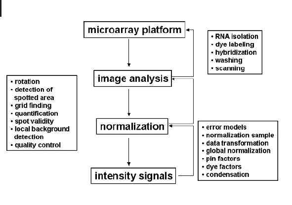
Fig. 9.1 Scheme of basic data capture modules

consisting of the microarray platform, image

analysis, and normalization. The entire process

estimates for each gene the concentration in the

target sample material by assigning a numerical

value to the gene’s representative on the array

(probe). It is assumed that this process (gene

concentration to probe signal) is approximately

linear. The bioinformatics modules in this pro-

cess model the factors of influences not inherent

in the probe-target interactions and try to elimi-

nate those influence factors for further analysis.

Boxes describe the different tasks in detail.

mation of the software (Wierling et al. 2002). However, for noisy images that show a

very irregular structure, manual methods might be the best choice (Fig. 9.2b).

9.1.2.3 Signal Validity

Signal validity has two tasks – the detection of spot artifacts (e.g., overshining of two

spots, background artifacts, irregular spot forms, etc.) and judgment on the detection

limit, i.e., whether the spot can reasonably be detected and thus if the gene is ex-

pressed in the tissue of interest or not. Spot artifacts are identified by applying mor-

phological feature recognition criteria such as circularity, regularity of spot form,

and background artifact detection methods. In the Affymetrix oligo-chip design, spot

validity is often judged by comparison of the PM/MM (perfect-match/mismatch)

pairs using a statistical test. Each gene is represented on the chip by a set of n oligo-

nucleotides (~20mers) that are distributed across the gene sequence (PM

,…,PM

For each perfect match, PM

, there is an oligonucleotide next to it, MM

, with a cen-

tral base pair mismatch in the original PM sequence (Fig. 9.2c). This value serves as

a local background for the probe. For each gene the perfect matches and the mis-

matches yield two series of values, PM

,…,PM

and MM

,…,MM

, and a Wilcoxon

rank test can be calculated for the hypothesis that the two signal series are equal or

not (cf. Section 3.4). If the P-value is low, this indicates that the signal series have sig-

nificantly higher values than the mismatch signal series, and thus it is likely that the

corresponding gene is expressed in the tissue. Conversely, if the P-value is not signif-

icant, then there is no great difference in PM and MM signals, and thus it is likely

that the gene is not expressed. In order to calculate a single expression value to the

probe, it has been assumed that the average of PM-MM differences is a good estima-

tor for the expression of the corresponding gene:



j1

PM

 MM



Here, y

corresponds to the ith gene and PM

and MM

are the jth perfect-match

and mismatch probe signals for gene i. This use of the mismatches for analysis has

been criticized. It has been reported that the MM signals often interact with the tran-

script and thus produce high signal values (Chudin et al. 2001). This fact is known

as cross-hybridization and is a severe practical problem. It has yielded to alternative

computation of the local background, e.g., by evaluating local neighborhoods of low

expressed probes (background zone weighting) (Draghici 2003).

In cDNA arrays, such types of significance tests for signal validity cannot be per-

formed on the spot level because, most commonly, each cDNA is spotted only a

small number of times so that there are not enough replicates for performing a test.

Instead, this procedure can be carried out on the pixel level. Here, for each spot a

local background area is defined, e.g., by separating foreground and background pix-

els by the segmentation procedure or by defining specific spot neighborhoods (cor-

ners, rings, etc.) as the local background. Alternatively, the signals can be compared

on the spot level to a negative control sample. For example, several array designs in-

corporate empty positions on the array (i.e., no material was transferred). The scan-

293

9.1 Data Capture

294

9 Analysis of Gene Expression Data

(a)

(b)

(c)

(d)

ning and image analysis will assign each such position a small intensity level that

corresponds to the local background. For each regular spot, a certain probability can

then be calculated that the spot is different from the negative sample (Fig. 9.2 d).

This can be done by outlier criteria or by direct comparison to the negative sample

(Kahlem et al. 2004).

Signal validity indices can be used as an additional qualifier for the expression ra-

tio. Suppose we compare a gene’s expression in two different conditions (A and B)

and then we distinguish four cases (1 = signal is valid, 0 = signal is invalid):

A B Ratio Interpretation Possible marker

1 1 Valid Gene expression is detectable in both conditions. Yes

1 0 Invalid Gene expression is detectable in condition A but not in B. Yes

0 1 Invalid Gene expression is detectable in condition B but not in A. Yes

0 0 Invalid Gene expression is not detectable in both conditions. No

Probes belonging to the fourth case should be removed from further analysis

since they represent genes that either are not expressed in both conditions or cannot

be detected using the microarray procedure (possibly a very low number of mole-

cules). This will occur fairly often in practice since only a part of the genes on the ar-

ray will be actually activated in the tissue under analysis. The other three cases might

reveal potential targets, but the expression ratio is meaningful only in the first case,

where both conditions generate valid signals.

295

9.1 Data Capture

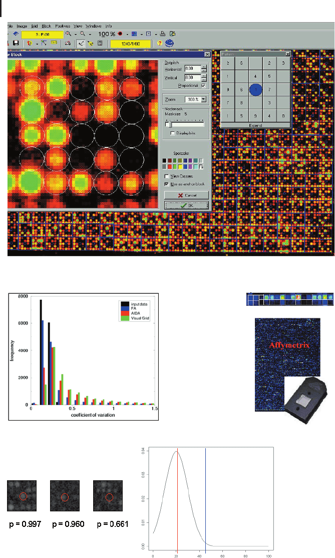
Fig. 9.2 Image analysis and data acquisition.

(a) Visualization of individual sub-grid adjust-

ment with Visual Grid (GPC Biotech AG). Spot-

ting patterns show the geometry of the cDNAs

organized in sub-grids. Local background can be

assigned to each spot by defining specific neigh-

borhoods. (b) Image analysis was performed

with three image analysis programs classified by

manual (green bars), semiautomated (red bars),

and automated (blue bars) procedures on simu-

lated data. The purpose of the simulation was to

compare the reproducibility of the signals by re-

plicated analysis of perturbed signals (CV value).

The histogram shows the frequencies (y-axis)

over the range of the CV (x-axis). (c) Affymetrix

geometry employs successive printing of gene

representatives (oligonucleotide probes). Ap-

proximately 20 different oligonucleotides that

are spread across the gene sequence are immo-

bilized (perfect matches), with each PM having

a one-base-pair mismatch (MM) next to it that

is an estimator for the local background. The

pair PM-MM is called a probe pair. The whole

set of PM-MM pairs for the same gene is called

a probe set. After image analysis the feature

values are condensed to a single value reflecting

the gene’s concentration in the target sample.

(d) Spot validity can be judged by a negative

control sample distributed on the array. After

quantification a small, nonzero intensity is as-

signed to each of these empty spots, reflecting

the amount of background signal on the array.

Since these positions are spread uniformly over

the array, the distribution of these signals re-

flects the distribution for signal noise for this ex-

periment and is an indicator of whether signals

are at the background level or reflect reliable ex-

pression levels. If the cumulative distribution

function for the spot’s signal is close to one

(blue line), this indicates that the cDNA is ex-

pressed in the tissue, whereas low values reflect

noise (red line). In practice cDNAs are consid-

ered “expressed” when their signal exceeds a

proportion above 0.9, a threshold consistent

with the limit of visual detection of the spots.

9.1.3

Pre-processing

The task of data pre-processing (or normalization) is the elimination of influence

factors that are not due to the probe-target interaction, such as labeling effects (dif-

ferent dyes), background correction, pin effects (spotting characteristics), outlier de-

tection (cross-hybridization of oligonucleotide-probes), etc. Many different algo-

rithms and methods have been proposed to fulfill these tasks. Rather than listing

these different methods, we will concentrate here on describing some common fun-

damental concepts. Data normalization has become a major research component in

recent years, resulting in many different methods that claim specific merits. A re-

view on normalization methods is given by Quackenbush (2002).

The purpose of pre-processing methods is to make signal values comparable across

different experiments. This involves two steps: the selection of a set of probes (the nor-

malization sample) and the calculation of numerical factors that are used to transform

the signal values within each experiment (the normalization parameters). The selec-

tion of a normalization sample is commonly implicitly based on the assumption that

the expression for the same probe in the normalization sample will not vary across ex-

periments for biological reasons. Different methods have been proposed for that pur-

pose, including (1) housekeeping genes, (2) selected probes whose mRNA is spiked to

the labeled target sample in equal amounts, and (3) numerical methods to select a set

of non-varying probes across the batch of experiments. While the first two cases in-

volve additional biological material, the third is directly based on the probes of inter-

est. Numerical methods try, for example, to calculate a maximal normalization sample

by so-called maximal invariant sets, i.e., maximal sets of probes whose signals have

the same rank order (compare Section 3.4) across all experiments under analysis, or

by applying an iterative regression approach (Draghici 2003).

9.1.3.1 Global Measures

The weakest transformation of data is given by estimating global factors to eliminate

multiplicative noise across arrays. A very robust procedure calculates the median sig-

nal of each array and determines a scaling factor that equalizes those medians. In

the next step this scaling factor is applied to each individual signal to adjust the raw

signals.

Alternatively, an iterative regression method can be applied to normalize the ex-

perimental batch. Assume we have two experiments; then, this algorithm reads as

follows (compare Section 3.4.4):

1. Apply a simple linear regression fit of the data from the two experiments.

2. Calculate the residual.

3. Eliminate those probes that have residuals above a certain threshold.

4. Repeat steps 1–3 until the changes in residuals are below a certain threshold.

A batch of more than two experiments can be normalized with this approach by

comparing each single experiment with a pre-selected experiment or with the in

296

9 Analysis of Gene Expression Data

silico average across the entire batch. Global measures can be used for normalizing

for overall influence factors that are approximately linear. Nonlinear and spatial ef-

fects (if present) are not addressed by these methods.

9.1.3.2 Linear Model Approaches

Linear model approaches have been used for cDNA arrays as well as for oligo chips.

The most common approaches of normalization using linear models are the models

of Kerr et al. (2000) and Li and Wong (2001).

A model for a spotted microarray developed by Kerr et al. (2000) defines several in-

fluence factors that contribute to artificial spot signals. The model reads

log y

ijkl

b  a

 d

 v

 g

 ag

 vg

 e

ijkl

: (9-1)

This model (cf. Section 3.4.3) takes into account a global mean effect, b, the effect of

the array i, and the effect of the dye j. v

is the effect of variety k, i.e., the specific cDNA

target sample, and g

is the effect of gene l. e

ijkl

is the random error assumed to be

Gaussian distributed with mean zero (compare Section 3.4.4). In a simpler model

there are no interactions. In practice, for example, there will be interactions between

gene and array effects, ag

, or between gene and sample effects, vg

. This can then be

solved with ANOVA methods incorporating interaction terms (Christensen 1996).

Li and Wong (2001) use a linear model approach for normalizing oligonucleotide

chips (d-chip). Here, the model assumes that the intensity signal of a probe j in-

creases linearly with the expression of the corresponding gene in the ith sample.

Equations for mismatch oligonucleotides and perfect-match oligonucleotides are

then given by

 a

 g

 e

 a

 g

 e : (9-2)

Here, a

is the background response for probe pair j, g

is the expression of the ith

gene, and v

and w

are the rates of increase for the mismatch and the perfect-match

probe, respectively. The authors developed a software package for performing analy-

sis and normalization of Affymetrix oligo chips that is available for academic re-

search (www.dchip.org).

9.1.3.3 Nonlinear and Spatial Effects

Spotted cDNA microarrays commonly incorporate nonlinear and spatial effects due

to different characteristics of the pins, the different dyes, and local distortions of the

spots.

A very popular normalization method for eliminating the dye-effect is LOWESS

(or LOESS), locally weighted polynomial regression (Cleveland 1979; Cleveland and

Devlin 1983). LOWESS is applied to each experiment with two dyes separately. The

data axis is screened with sliding windows and in each window a polynomial is fit

(compare Section 3.4.4)

297

9.1 Data Capture

y  b

 b

x  b

 ::: (9-3)

Parameters of the LOWESS approach are the degree of the polynomial (usually 1

or 2) and the size of the window. The local polynomials fit to each subset of the data

are almost always either linear or quadratic. Note that a zero-degree polynomial

would correspond to a weighted moving average. LOWESS is based on the idea that

any function can be well approximated in a small neighborhood by a low-order poly-

nomial. High-degree polynomials would tend to overfit the data in each subset and

are numerically unstable, making accurate computations difficult. At each point in

the dataset, the polynomial is fit using weighted least squares, giving more weight to

points near the point whose response is being estimated and less weight to points

further away. This can be achieved by the standard weight function, such as

wx

1  x  x



0; x

 1



; x

< 1 : (9-4)

Here x

is the current data point. After fitting the polynomial in the current win-

dow, the window is moved and a new polynomial is fit. The value of the regression

function for the point is then obtained by evaluating the local polynomial using the

explanatory variable values for that data point. The LOWESS fit is complete after re-

gression function values have been computed for each of the n data points. The final

result is a smooth curve providing a model for the data. An additional user-defined

smoothing parameter determines the proportion of data used in each fit. Large va-

lues of this parameter produce smooth fits. Typically smoothing parameters lie in

the range 0.25 to 0.5 (Yang et al. 2002).

9.1.3.4 Other Approaches

There are many other approaches to DNA array data normalization. One class of

such models employs variance stabilization (Durbin et al. 2002; Huber et al. 2002).

These methods address the problem that gene expression measurements have an ex-

pression-dependent variance and try to overcome this situation by a data transforma-

tion that can stabilize the variance across the entire range of expression. The trans-

formation step is usually connected with an error model for the data and a normali-

zation method (such as regression). The most popular of these variance stabiliza-

tions is the log transformation. However, the log transformation is difficult for small

expression values, which has led to the definition of alternative transformations.

A lot of the above-discussed normalization methods are included in the R statisti-

cal software package (www.r-project.org) and, particularly for microarray data evalua-

tion, in the R software packages distributed by the Bioconductor project, an open-

source and open-development software project to provide tools for microarray data

analysis (www.bioconductor.org).

298

9 Analysis of Gene Expression Data

9.2

Fold-change Analysis

The analysis of fold changes is a central part of transcriptome analysis. Questions of

interest are whether there are genes that can be identified as being differentially ex-

pressed when comparing two different conditions (e.g., a normal versus a disease

condition).

9.2.1

Planning and Designing Experiments

Whereas early studies of fold-change analysis were based on the expression ratio of

probes derived from the expression in a treatment and a control target sample, it has

been a working standard to perform experimental repetitions and to base the identi-

fication of differentially expressed genes on statistical testing procedures (recall Sec-

tion 3.4.3) judging the null hypothesis H

= m

versus the alternative H

= m

where m

, m

are the population means of the treatment and the control sample, re-

spectively. However, the expression ratio still carries valuable information and is

used as an indicator for the fold change. Strikingly, it is still very popular to present

the expression ratio in published results without any estimate of the error, and stu-

dies that employ ratio error bounds are hard to find (for an exception, see (Kahlem

et al. [2004]). It should be noted that the use of the fold change without estimates of

the error bounds is of very limited value. For example, probes with low expression va-

lues in both conditions can have tremendous ratios, but these ratios are meaningless

because they reflect only noise. A simple error calculation can be done as follows. As-

sume that we have replicate series for control and treatment series x

,…,x

and y

…, y

. A widely used error of the sample averages is the standard error of the mean





n 1n

i1





x

and S





m 1m

i1







: (9-5)

The standard error of the ratio can then be calculated as















: (9-6)

An important question in the design of such an experiment is how many repli-

cates should be used and what level of fold change can be detected. This, among

other factors, is dependent on the experimental noise. Experimental observations in-

dicate that an experimental noise of 15–25% can be assumed in a typical microarray

experiment. The experimental noise can be interpreted as the mean CV (compare

Section 3.4.2) of replicated series of expression values of the probes. The dependence

of the detectable fold change on the number of experimental repetitions and on the

experimental error has been discussed in several papers (Herwig et al. 2001; Zien

et al. 2003).

299

9.2 Fold-change Analysis